NBA Three Point Percentage Model "Mathy" Explanations

Data Tranformations

Due to variation in some of the variables that is not consistent throughout the data, I was immediately worried about heteroskedasticity and how this would impact my ability to get accurate coefficients for a regression.  I did a Bruesch-Pagan test for heteroskedasticity and got a p value of 0.0003155, meaning that there was significant evidence of heteroskedasticity in the data.  Because of this, I had to apply a transformation on the data.  I used a box-cox transformation, using the machine learning function “preProcess” to try to fix this heteroskedasticity.  The Breusch-Pagan test value was now greater than 0.05, meaning that heteroskedasticity in the data was now unlikely.  While heteroskedasticity and collinearity are both problems in this data, I was not too worried about their impact in the final regression because these problems would affect the standard errors much more than the coefficients, meaning that it wouldn’t impact the model’s predictive value.

Bayesian Three Point Percentage

One struggle that’s involved with projecting NBA three point shooting is the variation in three point attempts among NBA players.  Some players have a significant sample size of thousands of shots from behind the arc, while others (like A.J. Hammonds, who is 5-10 from three in his career) have very limited sample sizes and therefore their percentages do not accurately reflect their shooting ability.  Therefore, I used a Bayesian statistics method described in this article.  Feel free to read the article to see a more full explanation, but put simply this method uses a regression of NBA three point percentage on NBA three point attempts as a prior to predict NBA three point percentage.  As it states in the above article, the formula for this new stat (Bayesian three point percentage), is “is (α+3-Point Makes)/(β+ 3-Point Attempts), where α and β are prior parameters set up by regressing 3-point percentage on 3-point attempts.” In this equation, α is equal to the player’s predicted three point percentage times 100 and β is equal to 100.  I added in the variable “NBA three point attempts per min” to the right side of the regression, and used the above equation. I did this so that players who play limited minutes but take a lot of threes get credit for their three point attempts.  This formula does not alter three point percentages much for players with a significant amount of attempts (such as Steph Curry or Damian Lillard), but does for players with very few attempts.  This new stat became the dependent variable in my regression.  Later in the process, I also created the same stat for college three point percentage (Bayesian college three point percentage) which was used as one of the independent variables in the regression.

Final Weighted Regression

The process of finding the ending regression involved a lot of steps that I don’t have enough time to explain fully.  Instead, I’m just going to go over the final regression and give a synopsis of how I got there.  Here is a picture of the final regression:

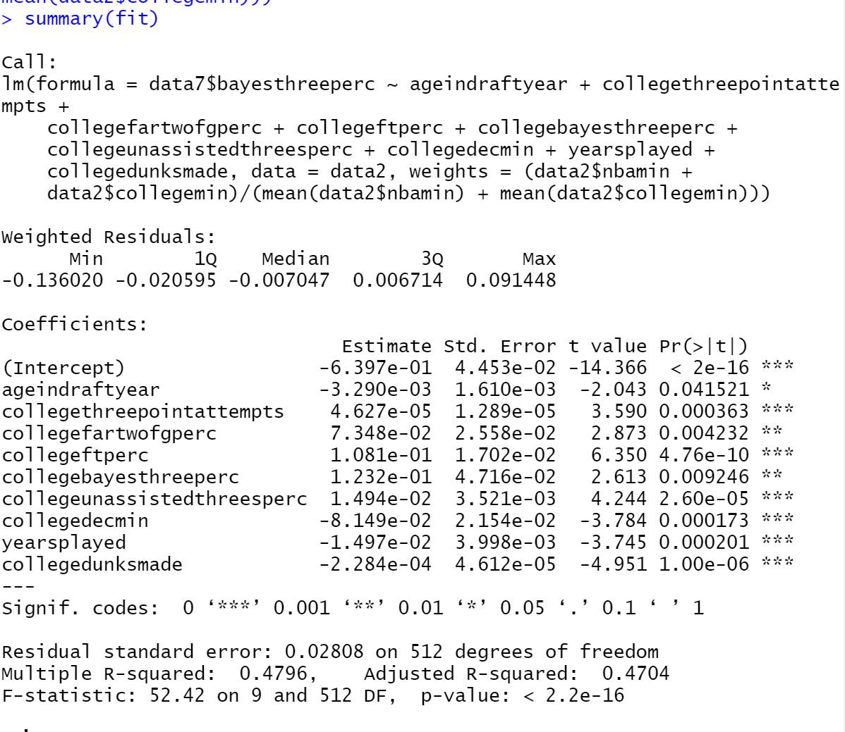
I tried several different regressions with many different combinations of variables before eventually finding which variables and regression type to stick with.  I mainly used regular multiple least squared regressions, ridge regressions (a regression used for data with multicollinearity), and weighted least squared regressions.   These 9 variables showed up as consistently statistically significant in the regressions I used, and therefore they were included in the final model.  The scaled average residual was 0.0355.  This average residual value means that the model was on average predictive of a players NBA three point percentage within 4 percentage points.  The Adjusted R-Squared value is 0.4704, showing a moderate relationship between the independent variables and the dependent variable. The final weights that were used were the z scores of combined NBA and college minutes for each player (meant to give players with a higher sample size more weight in the model).  One of the most interesting outcomes was the inclusion of “collegedunksmade” as a variable in the final regression.  This variable showed up as consistently statistically significant in different types of regressions and with different variables involved.  There’s a couple of possible explanations for its inclusion.  In my opinion, the most likely ones are that it’s a representation of athleticism or liking of shots near the rim compared to jump shots.  Most of the other variables are fairly unsurprising.  If an inference mindset had been used when looking at this data, there would be some more clear conclusions about which variables were most important towards predicting NBA three point percentage.  Because this route was not taken, I can’t say much about the influence of individual variables on the overall model.  Please comment if you have any questions on specifics of this project!